The purpose of the experiment using complex numbers with FreeMat.
Procedure:
A1 = 3+2j
A2 = -1+4j
B = 2-2j
1: Solve C = (A1 * B)/A2
2.
3.1.
3.2.
4.
Conclusion:
FreeMat works well with Complex Number.
Sunday, May 19, 2013
Wednesday, May 15, 2013
MOSFET Control of an Electric Motor
The objective of the experiment is to use a MOSFET to obtain a stable speed control.
Procedure:
Part 1:
We built the circuit below.
Using the pot, we were able to control the speed of the motor by adjusting amount of voltage through the motor.
Part 2:
We replace the pot with a Function Generator.
The FG produces Square Waves, and duty cycle was on.
Displaying the speed control by increasing and decreasing duty cycles.
Questions:
The motor rotates faster with a larger duty cycle.
The graph is the on/off times of the square function.
The time required to decelerate is 0.7s.
The voltage is 0.16 V at 30%
The converter allows a smooth speed control.
T = 1/110 = 9.1ms
Conclusion:
The lab was a success. Both ways controlled voltage, but part 2's method allowed for better speed control than part 1 with the pot.
Procedure:
Part 1:
We built the circuit below.
Using the pot, we were able to control the speed of the motor by adjusting amount of voltage through the motor.
Part 2:
We replace the pot with a Function Generator.
The FG produces Square Waves, and duty cycle was on.
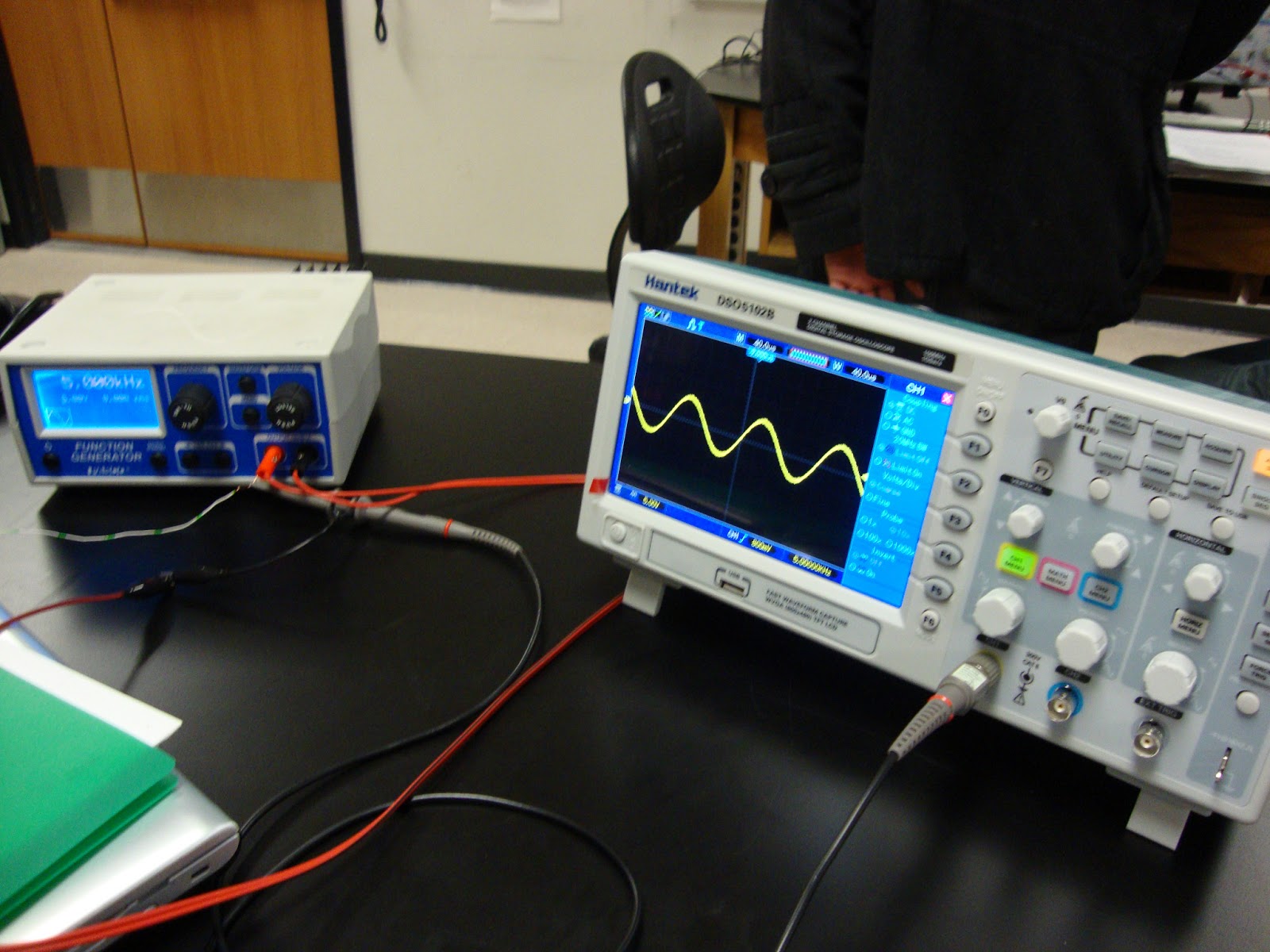
| We see how the voltage on the motor acts with the Oscilloscope. |
Displaying the speed control by increasing and decreasing duty cycles.
Questions:
The motor rotates faster with a larger duty cycle.
The graph is the on/off times of the square function.
The time required to decelerate is 0.7s.
The voltage is 0.16 V at 30%
| The voltage of motor at 30% of the maximum. |
T = 1/110 = 9.1ms
Conclusion:
The lab was a success. Both ways controlled voltage, but part 2's method allowed for better speed control than part 1 with the pot.
Sunday, May 5, 2013
Second Order Circuit Tutorial
The object of this lab is to study and practice second order circuits through an online tutorial.
Procedure:
We work on the tutorial and screenshot every answer.
Conclusion:
The lab was successful. It showed how simple solving Second Order Circuits were when broken down to many pieces.
Procedure:
We work on the tutorial and screenshot every answer.
Conclusion:
The lab was successful. It showed how simple solving Second Order Circuits were when broken down to many pieces.
Tuesday, April 30, 2013
Oscilloscope 101
The objective of the lab is to learn, use, and anaylze an oscilloscope.
Procedure:
We connect the oscilloscope with a frequency generation.
Exercise 1: Sinusoid
Once the trigger was set, we took measurements.
Period = 0.2 ms
Peak to Peak = 11.4 V
Zero to Peak = 5.8 V
Anticipated RMS = 3.53 V
Using DMM to take Voltage values
VDC = 0.026 mV
VAC = 3.35 V
The VAC is close to our anticipated RMS value.
Exercise 2: Include DC Offset
We add an offset of 2.5 V, and another one at 5V
The difference is that we can see the offset in DC coupling while nothing changes in AC.
2.5V offset measurements:
VDC = 2.51 V
VAC = 3.37 V
The VDC shows the offset in the output like the graph while the offset does not affect VAC.
Exercise 3: Square Wave with offset
VDC = 10 mV
VAC = 5.34 V
The measured value was close to the theoretical VAC = 5 V.
Exercise 4: Mystery Signal
DC Voltage = 448 mV
f = 70.42 Hz
Pk-Pk = 940 mV
Conclusion:
The lab was a success showing that it is more useful to use a digital oscilloscope to analyze waves than the heavy traditional ones.
Procedure:
We connect the oscilloscope with a frequency generation.
Exercise 1: Sinusoid
![]() |
| f = 5 kHz, V = 5V |
Period = 0.2 ms
Peak to Peak = 11.4 V
Zero to Peak = 5.8 V
Anticipated RMS = 3.53 V
Using DMM to take Voltage values
VDC = 0.026 mV
VAC = 3.35 V
The VAC is close to our anticipated RMS value.
Exercise 2: Include DC Offset
We add an offset of 2.5 V, and another one at 5V
![]() |
| DC Coupling at 5V |
![]() |
| AC Coupling at 5V |
2.5V offset measurements:
VDC = 2.51 V
VAC = 3.37 V
The VDC shows the offset in the output like the graph while the offset does not affect VAC.
Exercise 3: Square Wave with offset
VDC = 10 mV
VAC = 5.34 V
The measured value was close to the theoretical VAC = 5 V.
Exercise 4: Mystery Signal
![]() |
| Mystery Signal |
f = 70.42 Hz
Pk-Pk = 940 mV
Conclusion:
The lab was a success showing that it is more useful to use a digital oscilloscope to analyze waves than the heavy traditional ones.
Monday, April 22, 2013
Capacitor Charging/Discharging
The purpose of the experiment is to learn how to control capacitor charge and discharge times using a nonideal case.
Prelab:
We first build the Thevenin expressions for the charge and discharge circuits below to use later.
Charging: R_th = R_leak*R_charg/(R_leak + R_charg), V_th = R_leak*V_s/(R_charg + R_leak)
Discharge: R_th = R_leak*R_dischar/(R_leak + R_dischar), V_th = 0.
The setup is to use 9V to charge for 20s with 2.5 mJ, and discharge the 2.5 mJ in 2s.
Doing some math, we find:
C = 2*U/V^2 = 0.0617 mF
Charging: 5tau_c = 20s
R_c = 4/C = 64.8 kΩ
The power P_c = V^2/R_c =1.25 mW which is under the limit of 1W.
Discharging: 5tau_d = 2s
R_d = 2/(5*C) = 6.48 kΩ
The power P_d = 12.42 mW which is under the limit of 1W.
Procedure:
We build the circuit according to our values.
Analysis:
Logger pro was used to measure the change in voltage over time.
The peak voltage V_f = 8.25 V due logger pro's limit of 8Vs and the effect of the R_leak.
The time is estimated to be around 18s.
R_leak = R_charge /(V_s/V_f - 1) = 712.8 kΩ
Starting from V_f, the discharge time is around 2s.
Questions:
Using the Thevenin equations,
1. R_cth = 59.4 kΩ, V_cth = 8.25V
2. R_dth = 6.42 kΩ, V_dth = 0V
3. 0.6321*V_f = 5.215 V
5.215 V is around 4.6s
tau_c = RC = 4.6s
R = 4.6/C = 74.55 kΩ
Error = 15%
Practical Question:
1. U = (1/2)CV^2
C_eq = 2*U/V^2 = 2*160*10^6/(15*10^3)^2 = 1.42 F
2. 1/2C + 1/2C + 1/2C + 1/2C = 2C = C_eq
C = 1/2C_eq = 0.71 F
Conclusion:
The experiment was a success. The charge time was close to 20s, and discharge time was about 2s proving that it was possible to control the times.
Prelab:
We first build the Thevenin expressions for the charge and discharge circuits below to use later.
Charging: R_th = R_leak*R_charg/(R_leak + R_charg), V_th = R_leak*V_s/(R_charg + R_leak)
Discharge: R_th = R_leak*R_dischar/(R_leak + R_dischar), V_th = 0.
The setup is to use 9V to charge for 20s with 2.5 mJ, and discharge the 2.5 mJ in 2s.
Doing some math, we find:
C = 2*U/V^2 = 0.0617 mF
Charging: 5tau_c = 20s
R_c = 4/C = 64.8 kΩ
The power P_c = V^2/R_c =1.25 mW which is under the limit of 1W.
Discharging: 5tau_d = 2s
R_d = 2/(5*C) = 6.48 kΩ
The power P_d = 12.42 mW which is under the limit of 1W.
Procedure:
We build the circuit according to our values.
| Capacitors combined in parallel to reach desired value |
| Entire circuit with resistor boxes |
Logger pro was used to measure the change in voltage over time.
![]() |
| Capacitor charging |
The time is estimated to be around 18s.
R_leak = R_charge /(V_s/V_f - 1) = 712.8 kΩ
![]() |
| Capacitor discharge |
Questions:
Using the Thevenin equations,
1. R_cth = 59.4 kΩ, V_cth = 8.25V
2. R_dth = 6.42 kΩ, V_dth = 0V
3. 0.6321*V_f = 5.215 V
5.215 V is around 4.6s
tau_c = RC = 4.6s
R = 4.6/C = 74.55 kΩ
Error = 15%
Practical Question:
1. U = (1/2)CV^2
C_eq = 2*U/V^2 = 2*160*10^6/(15*10^3)^2 = 1.42 F
2. 1/2C + 1/2C + 1/2C + 1/2C = 2C = C_eq
C = 1/2C_eq = 0.71 F
Conclusion:
The experiment was a success. The charge time was close to 20s, and discharge time was about 2s proving that it was possible to control the times.
Wednesday, April 17, 2013
Op Amps II
The purpose of the lab is explore the effects of a varying input voltages, and feedback resistors on the output voltage on an inverting Op Amp.
Procedure:
We first consider this simple circuit.
Using the pot, we varied V_in and recorded the output.
I_cc = 0.874 mA
I_ee = -0.981 mA
I_cc + I_ee = -0.107 mA
P_cc = V*I = 10.488 mW
P_ee = 11.772 mW
Next we add a 1k resistor like shown below
However, we only took measurements when V_in = 1V.
I_ee + I_cc = -0.1 mA
P_cc = 10.644 mW
P_ee = 11.844 mW
Bonus:
The gain becomes -5 when R_f = 50 kΩ
Measured R_f = 49.9 kΩ
I_ee + I_cc = -0.1 mA
Conclusion:
The results are as expected because the ratio of the feedback resistors gives a gain of -10. V_in does not change the gain, only the resistors. KCL held, so the experiment was a success. To get a gain of 5, the ratio of R_i:R_f had to be 1:5, therefore R_f = 50 kΩ.
Procedure:
We first consider this simple circuit.
|
Resistor
|
Nominal
Value
|
Meaured
Value
|
|
R_1
|
10
kΩ
|
9.91
kΩ
|
|
R_F
|
100
kΩ
|
97.7
kΩ
|
| Building the Circuit |
| Finished circuit with the 12V rails |
Using the pot, we varied V_in and recorded the output.
|
V_in
(Desired)
|
V_in
(Actual)
|
V_out
(Measured)
|
V_RF
(Measured)
|
I_op
(Calculated)
|
|
0.25
V
|
0.24
V
|
-2.41
V
|
2.46
V
|
-0.0246
mA
|
|
0.5
V
|
0.50
V
|
-4.90
V
|
4.87
V
|
-0.0502
mA
|
|
1.0
V
|
1.00
V
|
-10.04
V
|
9.86
V
|
-0.1028
mA
|
I_cc = 0.874 mA
I_ee = -0.981 mA
I_cc + I_ee = -0.107 mA
P_cc = V*I = 10.488 mW
P_ee = 11.772 mW
Next we add a 1k resistor like shown below
| Part 2 Circuit Diagram |
| The final circuit |
However, we only took measurements when V_in = 1V.
|
V_in
(Desired)
|
V_out
(Measured)
|
V_RF
(Measured)
|
I_op
(Calculated)
|
I_cc
(Measured)
|
I_ee
(Measured)
|
|
1.0
V
|
-9.99
V
|
9.72
V
|
-0.102
mA
|
0.887
mA
|
-0.987
mA
|
I_ee + I_cc = -0.1 mA
P_cc = 10.644 mW
P_ee = 11.844 mW
Bonus:
| R_f was swapped with a variable resistor |
Measured R_f = 49.9 kΩ
|
V_in
(Desired)
|
V_out
(Measured)
|
V_RF
(Measured)
|
I_op
(Calculated)
|
I_cc
(Measured)
|
I_ee
(Measured)
|
|
1.0
V
|
-5.03
V
|
4.99
V
|
-0.101
mA
|
0.885
mA
|
-0.985
mA
|
I_ee + I_cc = -0.1 mA
Conclusion:
The results are as expected because the ratio of the feedback resistors gives a gain of -10. V_in does not change the gain, only the resistors. KCL held, so the experiment was a success. To get a gain of 5, the ratio of R_i:R_f had to be 1:5, therefore R_f = 50 kΩ.
Subscribe to:
Comments (Atom)


